
Data
All available public drilling data were analyzed to create the porosity and permeability maps. These are data from wells that are at least 5 years old, supplemented by more recent geothermal wells that have been made public earlies than after 5 years because the projects for which they have been collected have used RVO's Guarantee Fund. More data are available for porosity (~2160) than for permeability (~1100) (onshore, all aquifers). Not all data points were used to calculate the maps. The main reason for not using a data point is when the values is anomalous, considered not representative of the regional map image, or the data point is based on an unreliable measurement.
Porosity
Multiple porosity analyses may have been made for an aquifer encountered in a borehole. For the selection of data points to be used for interpolation, an selection order was applied based on the type of analysis shown below. The first is generally considered the most accurate and the last the least accurate: The order can be specified in the workflow.
- Petrophysical analysis
- LogQM average calibrated to core plug analysis data
- Petrophysical analysis of the ‘pay zone’
- Core plug analysis average
- LogQM average, not calibrated with core plug analysis data
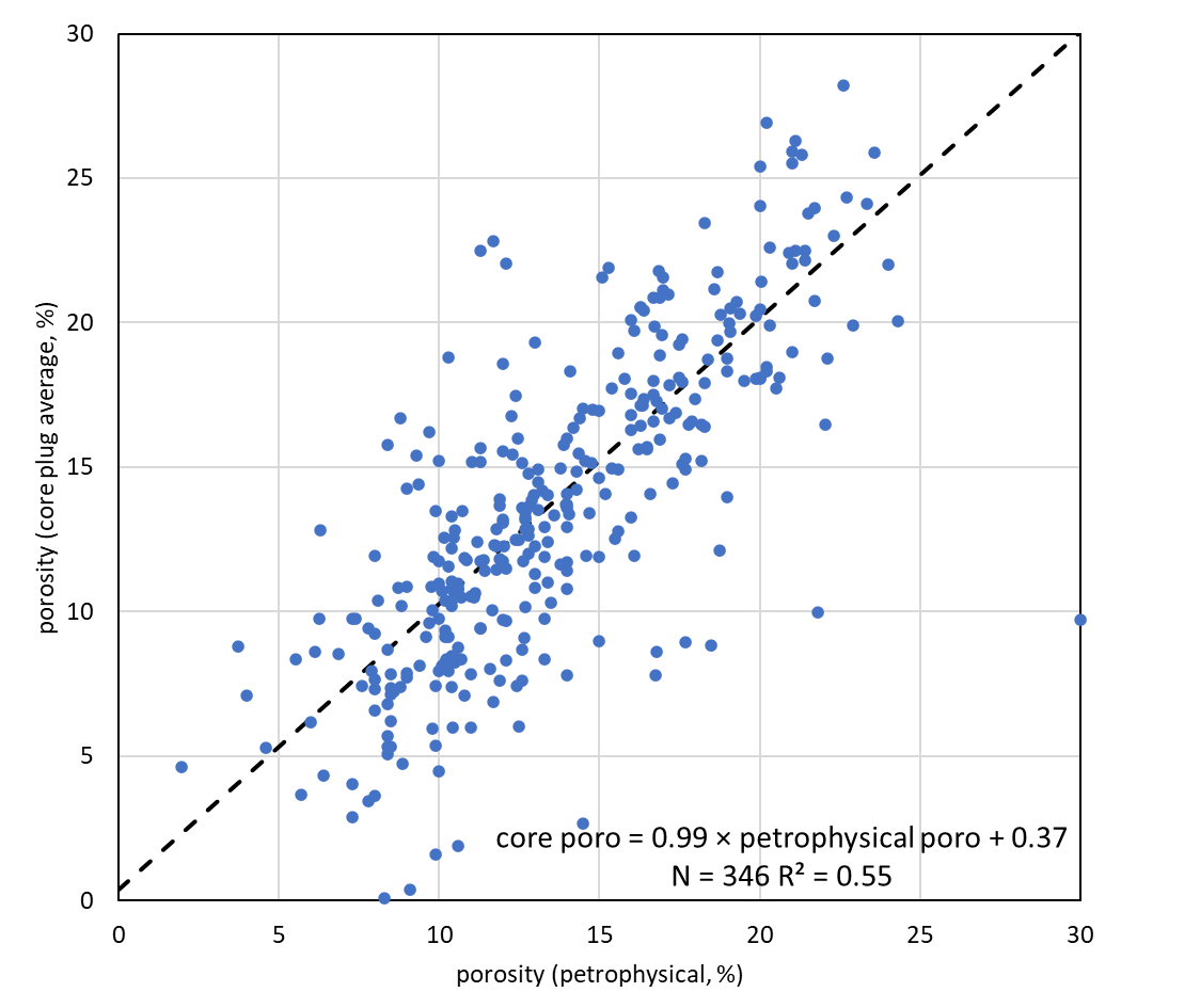
Most porosity data are from petrophysical analyses (1152) and core plug averages (1445). Both petrophysical porosity and core plug averages are available from 346 wells (Figure 3). On average, both match reasonably well, but the R² is low (0.55). When only boreholes with at least 20 core plug measurements are considered, it does become higher: 0.64.
Permeability
For permeability, as for porosity, several analytical results may be available for a single aquifer in a borehole. The possible types of analysis are:
- Welltest analysis
- Petrophysical analysis
- LogQM average
- Core plug analysis average
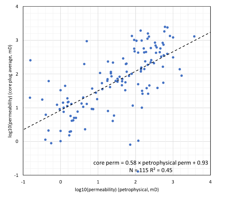
Most permeability data come from petrophysical analyses (422) and core plug averages (1384). Both petrophysical porosity and core plug averages are available from 131 wells (Figure 3). Compared with porosity (Figure 3), it is noticeable in Figure 4 that both bias and scatter are larger (R² = 0.45).
Maps
Porosity
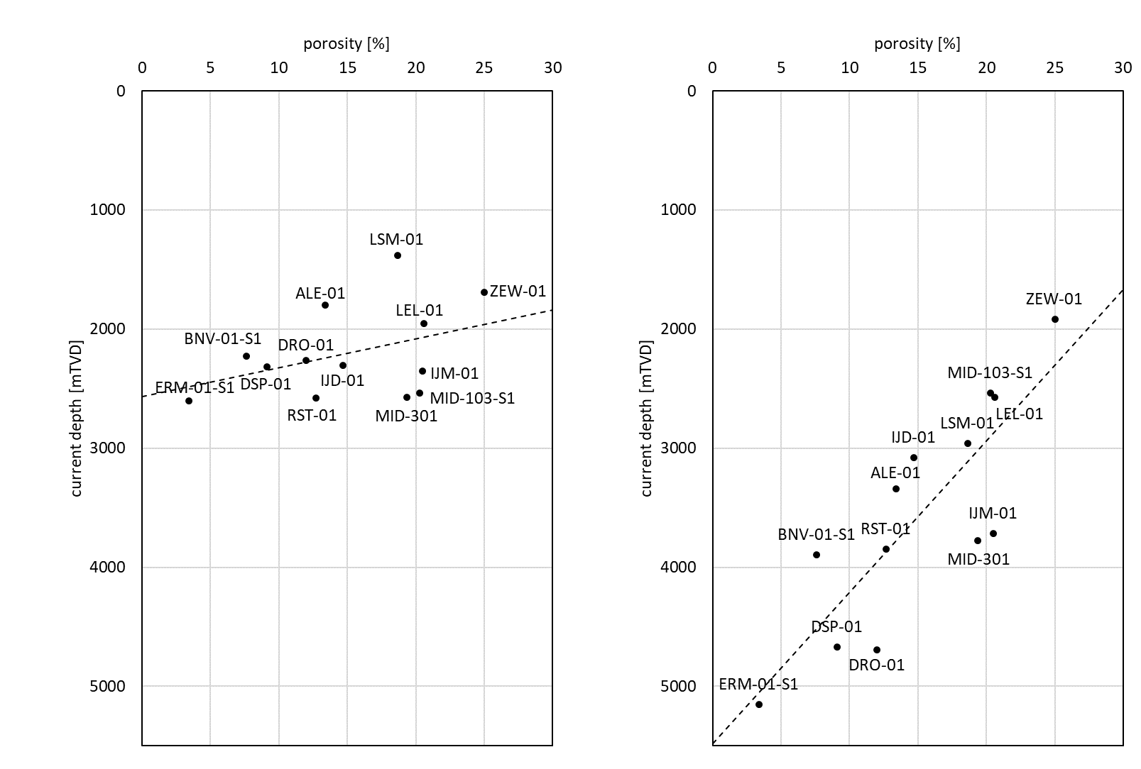
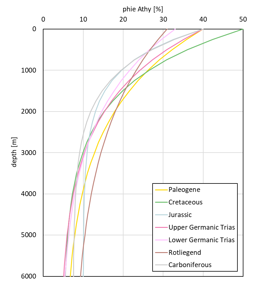
Porosity generally decreases with increasing burial depth, and is therefore strongly correlated with it. When a deeply buried aquifer with reduced porosity is inverted, the porosity will remain at the low level. Therefore, the workflow first calculated a trend porosity map by combining the maximum burial depth of the aquifer with a national-scale relationship between current porosity and maximum burial depth derived from the borehole porosity data. One porosity-depth relationship was determined for each main group (Paleogene, Cretaceous, etc.). The maximum burial depth was determined in a number of basin modelling studies (Nelskamp & Verweij 2012, Abdul Fattah & Verweij 2017, van Wees **North Holland**, Van Dalfsen et al. 2005, Bouroullec et al. 2019). As an illustration, Figure 5 shows the relationship between porosity and current depth, and maximum burial depths, for a number of selected boreholes in thecentral part of the Netherlands. There appears to be no relationship between porosity and current depth (R² = 0.15). For all boreholes, the current depth was then corrected to the maximum burial depth. For example, the Rotliegend in the Ermelo borehole is currently at about 2600 metres depth, but has been buried to about 5200 metres depth in the past. A clear relationship exists between porosity and maximum burial depth (R² = 0.70). Figure 6 shows the porosity-depth relationships used. Finally, the porosity map was calculated by calculating for each data point the difference with the trend porosity map and the porosity value of the data point (the residual), Kriging the residuals and adding them to the trend. Table 2 shows the used variogram settings (spherical variogram).
Table 2 Variogram parameters
| net to gross | permeability | porosity | |||||||
| layer | nugget | range | sill | nugget | range | sill | nugget | range | sill |
| N | 0.25 | 40000 | 4 | 0.2 | 10000 | 1 | 0.25 | 40000 | 4 |
| KN | 0.25 | 40000 | 4 | 0.2 | 10000 | 1 | 0.25 | 40000 | 4 |
| SL | 0.25 | 40000 | 4 | 0.2 | 10000 | 1 | 0.25 | 40000 | 4 |
| RN | 0.25 | 40000 | 4 | 0.2 | 10000 | 1 | 0.25 | 40000 | 4 |
| RB | 0.25 | 40000 | 4 | 0.2 | 10000 | 1 | 0.25 | 40000 | 4 |
| RO | 0.25 | 40000 | 4 | 0.2 | 10000 | 1 | 0.25 | 40000 | 4 |
| DC | 0.25 | 40000 | 4 | 0.2 | 10000 | 1 | 0.25 | 40000 | 4 |
Permeability
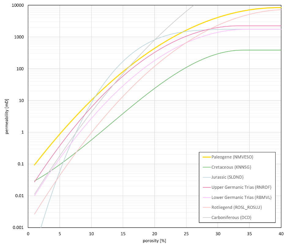
A trend permeability map was calculated by converting the porosity map using a porosity-permeability relationship (Figures7, 8). These relationships were determined per aquifer, or group of aquifers when considered relevant (e.g. for the Carboniferous and Paleogene aquifers), from core plug data. From the core plug measurements, the Swanson's Mean of the permeability was determined for each porosity point (Figure 7). A regression line representing the relationship between porosity and permeability was fit through these points. The best fit is generally obtained with a second-degree curve:
ln(k)=aφ²+bφ+c (1)
with:
k = permeability [mD]
φ = porosity[(%]
a, b, c = constants
When insufficient core plug measurements are available, the regression line cannot be determined accurately. In the example of Figure 7, this is the case for porosities less than ~7 and exceeding~32%. To avoid high porosity values leading to unrealistically high permeability values, the curve should be defined in such a way that it flattens at high porosity values. The maximum permeability value should be chosen based on geological knowledge of the aquifer. The exact location of the curve at very low porosity values is less relevant because very low porosities generally correspond to permeability values that are not important for geothermal exploration.
A permeability map was constructed by calculating for each data point the difference in permeability between the trend map and the value of the data points (the residual), Kriging this and adding the residual map to the trend.
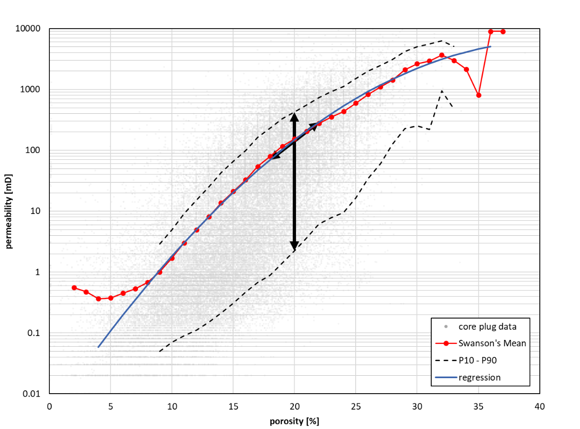
Among the properties that determine the geothermal potential of the aquifer, permeability is the most important one. Therefore, to determine the uncertainty of the calculated geothermal potential, it is necessary to know the uncertainty of the calculated permeability. In Figure 7, the height of the point cloud, for example in the form of the P90 and P10 curves, is a measure of the uncertainty of the permeability at a given porosity. For example, when the porosity is 20%, the P90-P10 range is between 2 and 400 mD, and the expectation (Swanson's Mean) 150 mD (black vertical arrow). However, this bandwidth is based on core plug measurements and overestimates the uncertainty in the average permeability of the aquifer, because the spread between the individual permeabilities of the core plugs is much larger than the uncertainty in the average permeability of the aquifer (the spread in the permeability of the core plugs is averaged out over the aquifer). Therefore, the blue regression line, which is fitted using the Swanson's Means, is used. If the uncertainty in porosity at a given location (following from the Kriging of porosity and expressed as the standard deviation), is, for instance, 2%, the expected permeability is between 70 and 290 mD (black sloping arrow). The standard deviation of the trend permeability can be calculated from that of the porosity (stdev(φ)) and the slope of the regression line as follows:
stdev(ln(k) )=√((slope × stdev(φ))²)) = stdev(φ) × √slope (2)
with:
k = permeability [mD]
φ = porosity [%]
where the slope of the regression line for a second-degree regression is equal to 2a φ + b (the derivative). The stdev(φ) is the uncertainty of porosity integrated over the thickness of the formation in terms of its effect on permeability. The, the standard deviation of the Kriged residual permeability is added to the previously determined standard deviation of the trend permeability.
Dinantian
Too few porosity and permeability measurements are known from the Dinantian to enable the construction of a permeability map. The limestones of this unit have very low primary porosity and permeability. However, sometimes they do have secondary permeability due to dissolution (karst) and/or faulting. This permeability is spatially distributed very heterogeneously. The techniques used to calculate permeability maps of the other (clastic) aquifers are therefore unsuitable for the Dinantian.